Rotational dynamics Quickstart
Calculation of rotational (and generally ro-vibrational) dynamics proceeds in two main steps. At the first step, we obtain the molecular field-free rotational energies and wave functions, which we then use at the second step to form a basis for representing the time-dependent wavepacket or field-dressed states. The interaction of a molecule with field is described in terms of the multipole moments, e.g., the permanent dipole moment, polarizability, hyper-polarizability, quadrupole moment, etc. The matrix elements of these interaction tensors, defined with respect to the laboratory frame, are computed in the basis of the field-free wave functions. The molecule-field interaction potential is built as a sum of interaction tensors multiplied with field and the time-dependent Schrödinger equation is solved variationally.
Molecular field-free rotational solutions
[1]:
from richmol.rot import Molecule, solve, LabTensor
WARNING:absl:No GPU/TPU found, falling back to CPU. (Set TF_CPP_MIN_LOG_LEVEL=0 and rerun for more info.)
Here is an example for water molecule, using data obtained from a quantum chemical calculation
[2]:
water = Molecule()

# Cartesian coordinates of atoms
water.XYZ = ("bohr",
             "O",  0.00000000,   0.00000000,   0.12395915,
             "H",  0.00000000,  -1.43102686,  -0.98366080,
             "H",  0.00000000,   1.43102686,  -0.98366080)

# choose frame of principal axes of inertia
water.frame = "ipas"

# molecular-frame dipole moment (au)
water.dip = [0, 0, -0.7288]

# molecular-frame polarizability tensor (au)
water.pol = [[9.1369, 0, 0], [0, 9.8701, 0], [0, 0, 9.4486]]

# symmetry group
water.sym = "D2"

# rotational solutions for J=0..5
Jmax = 5
sol = solve(water, Jmin=0, Jmax=Jmax)

# laboratory-frame dipole moment operator
dip = LabTensor(water.dip, sol, thresh=1e-12) # neglect matrix elements smaller than `thresh`

# laboratory-frame polarizability tensor
pol = LabTensor(water.pol, sol, thresh=1e-12)

# field-free Hamiltonian
h0 = LabTensor(water, sol, thresh=1e-12)
Here, water.XYZ defines molecular geometry. By default, calculations are carried out for the main isotopologue. To specify a non-standard isotope, put the corresponding isotope number next to the atom label, for example, "O18" for \(^{18}O\) or "H2" for deuterium.
The properties water.dip and water.pol determine molecular-frame dipole moment and polarizability, respectively, defined with respect to the same frame as Cartesian coordinates of atoms in water.XYZ.
The orientation of molecular axes with respect to molecule (so-called molecular frame embedding) is determined by water.frame="ipas", in the present case we choose the inertial principal axes system.
The molecular symmetry group is specified in water.sym="D2", here we choose the \(D_2\) rotational symmetry group.
The variational solutions are obtained using solve function for a range of \(J\) quanta from Jmin to Jmax. It outputs a dictionary object sol[J][sym] for different values of \(J\) (Jmin..Jmax) and different symmetries (spanned by \(D_2\)).
LabTensor computes matrix elements of laboratory-frame dipole moment and polarizability tensors in the basis of rotational solutions sol. When LabTensor is applied to a molecule object, i.e. water in this case, it converts the field-free solutions sol into a laboratory-frame tensor, which is convenient (as shown later) for building the total molecule-field interaction Hamiltonian.
The field-free rotational energies and wave functions are contained in the dictionary object sol[J][sym] for different values of quantum number \(J\) (int) and different symmetries (str) of the \(D_2\) rotational group (water.sym="D2"). The rotational energies and assignments (by the \(J, k, \tau\) quantum numbers) can be printed out as following
[3]:
print("J  sym #    energy      J   k  tau  |leading coef|^2")
for J in sol.keys():
    for sym in sol[J].keys():
        for i in range(sol[J][sym].nstates):
            print(J, "%4s"%sym, i, "%12.6f"%sol[J][sym].enr[i], sol[J][sym].assign[i])
J  sym #    energy      J   k  tau  |leading coef|^2
0    A 0     0.000000 ['0' '0' '0' ' 1.000000']
1   B1 0    41.996372 ['1' '0' '1' ' 1.000000']
1   B2 0    36.931654 ['1' '1' '0' ' 1.000000']
1   B3 0    24.103743 ['1' '1' '1' ' 1.000000']
2    A 0    71.083285 ['2' '2' '0' ' 0.859287']
2    A 1   134.980252 ['2' '0' '0' ' 0.859287']
2   B1 0    80.074422 ['2' '2' '1' ' 1.000000']
2   B2 0    95.268576 ['2' '1' '0' ' 1.000000']
2   B3 0   133.752307 ['2' '1' '1' ' 1.000000']
3    A 0   206.063537 ['3' '2' '0' ' 1.000000']
3   B1 0   174.290919 ['3' '2' '1' ' 0.709733']
3   B1 1   283.750848 ['3' '0' '1' ' 0.709733']
3   B2 0   144.095391 ['3' '3' '0' ' 0.967197']
3   B2 1   283.558067 ['3' '1' '0' ' 0.967197']
3   B3 0   138.894101 ['3' '3' '1' ' 0.865893']
3   B3 1   211.791894 ['3' '1' '1' ' 0.865893']
4    A 0   225.839342 ['4' '4' '0' ' 0.897851']
4    A 1   316.682576 ['4' '2' '0' ' 0.534048']
4    A 2   487.795766 ['4' '0' '0' ' 0.612490']
4   B1 0   228.396486 ['4' '4' '1' ' 0.948500']
4   B1 1   381.957482 ['4' '2' '1' ' 0.948500']
4   B2 0   277.742376 ['4' '3' '0' ' 0.631211']
4   B2 1   383.258773 ['4' '1' '0' ' 0.631211']
4   B3 0   301.509448 ['4' '3' '1' ' 0.918683']
4   B3 1   487.770805 ['4' '1' '1' ' 0.918683']
5    A 0   419.313391 ['5' '4' '0' ' 0.859287']
5    A 1   611.004294 ['5' '2' '0' ' 0.859287']
5   B1 0   403.603021 ['5' '4' '1' ' 0.645844']
5   B1 1   509.913211 ['5' '0' '1' ' 0.363766']
5   B1 2   746.747028 ['5' '0' '1' ' 0.546915']
5   B2 0   332.465633 ['5' '5' '0' ' 0.941152']
5   B2 1   505.082745 ['5' '3' '0' ' 0.814480']
5   B2 2   746.744110 ['5' '1' '0' ' 0.869201']
5   B3 0   331.342554 ['5' '5' '1' ' 0.919955']
5   B3 1   449.307570 ['5' '1' '1' ' 0.527404']
5   B3 2   611.223709 ['5' '3' '1' ' 0.526614']
Here, \(k\) is quantum number of the rotational angular momentum projection onto the molecular \(z\) axis, \(\tau\) is rotational parity, defined as \((-1)^\tau\), and coefficient corresponds to the leading symmetric-top function in the wave function expansion. We can print second and third (and more) leading contributions by setting, e.g., sol[J][sym].assign_nprim = 3, for selected \(J\) and symmetry.
The matrix elements of laboratory-frame interaction tensors (multipole moments) in the basis of rotational solutions can be retrieved in dense or sparse matrix formats using tomat method, for example
[4]:
# X-component of dipole moment
mu_x = dip.tomat(form="full", cart="x")

# XZ-component of polarizability
alpha_xz = pol.tomat(form="full", cart="xz")

# field-free Hamiltonian
h0mat = h0.tomat(form="full", cart="0") # note cart="0" must be specified

print("matrix dimensions:", h0mat.shape)
print("dipole X:", mu_x)
print("\npolarizability XZ:", alpha_xz)
print("\nfield-free Hamiltonian:", h0mat)
matrix dimensions: (286, 286)
dipole X:   (0, 4)      (-9.739787996057844e-35-0.2975313540900633j)
  (0, 6)        (9.739787996057844e-35+0.2975313540900633j)
  (1, 8)        (-8.434903832060798e-35-0.25766971106437786j)
  (1, 30)       (1.3610889671164236e-34+0.2822630262715965j)
  (1, 32)       (-5.55662243994505e-35-0.11523339793653574j)
  (2, 7)        (-8.434903832060798e-35-0.25766971106437786j)
  (2, 9)        (-8.434903832060798e-35-0.25766971106437786j)
  (2, 31)       (9.624352384462173e-35+0.19959009995488255j)
  (2, 33)       (-9.624352384462173e-35-0.19959009995488255j)
  (3, 8)        (-8.434903832060798e-35-0.25766971106437786j)
  (3, 32)       (5.55662243994505e-35+0.11523339793653574j)
  (3, 34)       (-1.3610889671164236e-34-0.2822630262715965j)
  (4, 0)        (-9.739787996057844e-35+0.2975313540900633j)
  (4, 10)       (3.774036515276408e-33+0.20052055607190467j)
  (4, 11)       (1.887018257638204e-33+0.25694628736880804j)
  (4, 14)       (-1.5407439555097885e-33-0.08186217421921828j)
  (4, 15)       (-7.7037197775489426e-34-0.10489788255935238j)
  (5, 12)       (2.668646812397596e-33+0.14178944496574117j)
  (5, 13)       (1.334323406198798e-33+0.18168846219919157j)
  (5, 16)       (-2.668646812397596e-33-0.14178944496574117j)
  (5, 17)       (-1.334323406198798e-33-0.18168846219919157j)
  (6, 0)        (9.739787996057844e-35-0.2975313540900633j)
  (6, 14)       (1.5407439555097885e-33+0.08186217421921828j)
  (6, 15)       (7.7037197775489426e-34+0.10489788255935238j)
  (6, 18)       (-3.774036515276408e-33-0.20052055607190467j)
  :     :
  (281, 218)    (4.092359016461902e-34-0.11790707114366855j)
  (281, 219)    (2.7872077398459563e-33+0.002715814400525685j)
  (282, 125)    (1.725106954595315e-33-0.009616951979301387j)
  (282, 126)    (7.76059936224008e-34+0.25047611779505286j)
  (282, 211)    (-5.8843163600120894e-34-0.015243232013320441j)
  (282, 212)    (1.7674080268623158e-33+0.12240087289752385j)
  (282, 213)    (8.915633013702843e-35+0.0893487262800264j)
  (282, 217)    (-4.385910460700387e-34-0.011361634326195164j)
  (282, 218)    (1.3173481640143044e-33+0.09123222410139167j)
  (282, 219)    (6.645320493693625e-35+0.06659660855505366j)
  (283, 127)    (1.1901499371844318e-32-0.3077040054890197j)
  (283, 128)    (-4.343813211512369e-33+0.016409267103435588j)
  (283, 214)    (-1.6121605803088443e-33+0.0872890316266411j)
  (283, 215)    (7.447083925841683e-34-0.015906470987632797j)
  (283, 216)    (-3.461832680173917e-34+0.00041897802440189996j)
  (284, 127)    (4.198996431039597e-36-0.0955090392948147j)
  (284, 128)    (-8.814084036232769e-34+0.10263425886319406j)
  (284, 214)    (-7.743282799110597e-34-0.13026893601732828j)
  (284, 215)    (4.0923590164619015e-34-0.11790707114366854j)
  (284, 216)    (2.787207739845956e-33+0.0027158144005256847j)
  (285, 127)    (1.928728209466384e-33-0.010752079181034527j)
  (285, 128)    (8.676613860055167e-34+0.2800408130649915j)
  (285, 214)    (-4.385910460700386e-34-0.011361634326195164j)
  (285, 215)    (1.3173481640143042e-33+0.09123222410139167j)
  (285, 216)    (6.645320493693624e-35+0.06659660855505364j)

polarizability XZ:   (0, 12)    (-0.09755930791281402+1.8057681046450725e-17j)
  (0, 13)       (0.06342085177268478-1.1738844170858955e-17j)
  (0, 16)       (0.09755930791281404-2.7656900498342933e-17j)
  (0, 17)       (-0.06342085177268479+1.797905524878078e-17j)
  (1, 2)        (-0.07388558756618278+2.094568306496896e-17j)
  (1, 20)       (0.05441541601421423-1.0071988490044882e-17j)
  (1, 22)       (-0.06664500168804863+1.8893063305097118e-17j)
  (1, 44)       (-0.08632246206263056+1.5977803865361223e-17j)
  (1, 45)       (0.04962000720348973-9.184385198836739e-18j)
  (1, 48)       (0.04728075969108671-1.3403531597733845e-17j)
  (1, 49)       (-0.02717799724892017+7.704638150255837e-18j)
  (2, 1)        (-0.07388558756618274+1.3675808108356735e-17j)
  (2, 3)        (0.07388558756618276-2.0945683064968953e-17j)
  (2, 21)       (-0.038477509664737924+7.121971361343592e-18j)
  (2, 23)       (-0.03847750966473793+1.0907915185014462e-17j)
  (2, 46)       (-0.07720915726287547+1.4290982229642637e-17j)
  (2, 47)       (0.044381483660412925-8.21476385445675e-18j)
  (2, 50)       (0.07720915726287549-2.1887875443812853e-17j)
  (2, 51)       (-0.04438148366041293+1.2581621413938423e-17j)
  (3, 2)        (0.07388558756618277-1.3675808108356743e-17j)
  (3, 22)       (-0.06664500168804863+1.2335616247897587e-17j)
  (3, 24)       (0.054415416014214235-1.5426121591862876e-17j)
  (3, 48)       (-0.0472807596910867+8.75140359645158e-18j)
  (3, 49)       (0.027177997248920168-5.030494950219453e-18j)
  (3, 52)       (0.08632246206263058-2.447138868770695e-17j)
  :     :
  (282, 82)     (-0.005594986726938355+1.0356006816332482e-18j)
  (282, 83)     (0.03995640789989996-7.395707135018623e-18j)
  (282, 161)    (-0.014938631080207588+2.7650568775873082e-18j)
  (282, 162)    (0.04829207241148299-8.938591912295875e-18j)
  (282, 277)    (-0.002163831826599701+4.005131421987464e-19j)
  (282, 278)    (-0.008149889663058053+1.5084988941371748e-18j)
  (282, 279)    (0.04828854114931652-8.937938295462611e-18j)
  (282, 283)    (-0.0020736321669233442+5.878499933805838e-19j)
  (282, 284)    (-0.007810160269594571+2.214087308258947e-18j)
  (282, 285)    (0.046275625947500384-1.3118588166618726e-17j)
  (283, 163)    (-0.015488546540404154+2.866843146834073e-18j)
  (283, 164)    (-0.00015297646330733158+2.8315085880750557e-20j)
  (283, 280)    (-0.09752217726834075+1.805080837228675e-17j)
  (283, 281)    (-0.008152270401529797+1.508939555483566e-18j)
  (283, 282)    (-0.0020736321669233386+3.8381769078790187e-19j)
  (284, 163)    (-0.09432175240337505+1.745842766909103e-17j)
  (284, 164)    (0.0015139781134612853-2.8022886251533466e-19j)
  (284, 280)    (-0.008152270401529806+1.5089395554835656e-18j)
  (284, 281)    (-0.018974256644475697+3.512028548681794e-18j)
  (284, 282)    (-0.007810160269594571+1.4456168876888493e-18j)
  (285, 163)    (-0.03340379458613528+6.182855139938536e-18j)
  (285, 164)    (0.10798435668641816-1.9987299139023414e-17j)
  (285, 280)    (-0.0020736321669233442+3.838176907879013e-19j)
  (285, 281)    (-0.007810160269594571+1.4456168876888493e-18j)
  (285, 282)    (0.046275625947500384-8.565358974579855e-18j)

field-free Hamiltonian:   (1, 1)        (41.996371682354464-1.0413888945031573e-48j)
  (2, 2)        (41.996371682354464-1.0413888945031573e-48j)
  (3, 3)        (41.996371682354464-1.0413888945031573e-48j)
  (4, 4)        (36.93165361155496+2.8401161870723716e-32j)
  (5, 5)        (36.93165361155496+2.8401161870723716e-32j)
  (6, 6)        (36.93165361155496+2.8401161870723716e-32j)
  (7, 7)        (24.103743154821103+3.2964703713189847e-32j)
  (8, 8)        (24.103743154821103+3.2964703713189847e-32j)
  (9, 9)        (24.103743154821103+3.2964703713189847e-32j)
  (10, 10)      (71.0832845583496-1.2106702985004045e-30j)
  (10, 11)      0j
  (11, 10)      0j
  (11, 11)      (134.98025233911153+4.1322080999273885e-32j)
  (12, 12)      (71.0832845583496-1.2106702985004045e-30j)
  (12, 13)      0j
  (13, 12)      0j
  (13, 13)      (134.98025233911153+4.1322080999273885e-32j)
  (14, 14)      (71.0832845583496-1.2106702985004045e-30j)
  (14, 15)      0j
  (15, 14)      0j
  (15, 15)      (134.98025233911153+4.1322080999273885e-32j)
  (16, 16)      (71.0832845583496-1.2106702985004045e-30j)
  (16, 17)      0j
  (17, 16)      0j
  (17, 17)      (134.98025233911153+4.1322080999273885e-32j)
  :     :
  (261, 261)    (611.2237086086233-2.2968929053986172e-30j)
  (262, 262)    (331.34255364752323-6.923451621833251e-30j)
  (263, 263)    (449.3075695534758+1.9264598480804652e-30j)
  (264, 264)    (611.2237086086233-2.2968929053986172e-30j)
  (265, 265)    (331.34255364752323-6.923451621833251e-30j)
  (266, 266)    (449.3075695534758+1.9264598480804652e-30j)
  (267, 267)    (611.2237086086233-2.2968929053986172e-30j)
  (268, 268)    (331.34255364752323-6.923451621833251e-30j)
  (269, 269)    (449.3075695534758+1.9264598480804652e-30j)
  (270, 270)    (611.2237086086233-2.2968929053986172e-30j)
  (271, 271)    (331.34255364752323-6.923451621833251e-30j)
  (272, 272)    (449.3075695534758+1.9264598480804652e-30j)
  (273, 273)    (611.2237086086233-2.2968929053986172e-30j)
  (274, 274)    (331.34255364752323-6.923451621833251e-30j)
  (275, 275)    (449.3075695534758+1.9264598480804652e-30j)
  (276, 276)    (611.2237086086233-2.2968929053986172e-30j)
  (277, 277)    (331.34255364752323-6.923451621833251e-30j)
  (278, 278)    (449.3075695534758+1.9264598480804652e-30j)
  (279, 279)    (611.2237086086233-2.2968929053986172e-30j)
  (280, 280)    (331.34255364752323-6.923451621833251e-30j)
  (281, 281)    (449.3075695534758+1.9264598480804652e-30j)
  (282, 282)    (611.2237086086233-2.2968929053986172e-30j)
  (283, 283)    (331.34255364752323-6.923451621833251e-30j)
  (284, 284)    (449.3075695534758+1.9264598480804652e-30j)
  (285, 285)    (611.2237086086233-2.2968929053986172e-30j)
By default, the basis of field-free rotational solutions is spanned by \(J\) ranging from Jmin to Jmax (defined in solve), \(m=-J..J\), \(k=0..J\), and \(\tau=0,1\). The assignment of basis states by symmetric-top functions can be obtained using assign method
[7]:
assign_bra, assign_ket = h0.assign(form="full") # assignment of bra and ket states, i.e. `assign_bra` and `assign_ket` are equivalent in this case
assign = assign_bra

# print assignments for the first 20 states
for i in range(20):
    print(i, "J =", assign["J"][i], ", sym =", assign["sym"][i], ", m =", assign["m"][i], ", k =", assign["k"][i])
0 J = 0.0 , sym = A , m = 0 , k = ('0 0 0  1.000000', 0.0)
1 J = 1.0 , sym = B1 , m = -1 , k = ('1 0 1  1.000000', 41.996371682354464)
2 J = 1.0 , sym = B1 , m = 0 , k = ('1 0 1  1.000000', 41.996371682354464)
3 J = 1.0 , sym = B1 , m = 1 , k = ('1 0 1  1.000000', 41.996371682354464)
4 J = 1.0 , sym = B2 , m = -1 , k = ('1 1 0  1.000000', 36.93165361155496)
5 J = 1.0 , sym = B2 , m = 0 , k = ('1 1 0  1.000000', 36.93165361155496)
6 J = 1.0 , sym = B2 , m = 1 , k = ('1 1 0  1.000000', 36.93165361155496)
7 J = 1.0 , sym = B3 , m = -1 , k = ('1 1 1  1.000000', 24.103743154821103)
8 J = 1.0 , sym = B3 , m = 0 , k = ('1 1 1  1.000000', 24.103743154821103)
9 J = 1.0 , sym = B3 , m = 1 , k = ('1 1 1  1.000000', 24.103743154821103)
10 J = 2.0 , sym = A , m = -2 , k = ('2 2 0  0.859287', 71.08328455834958)
11 J = 2.0 , sym = A , m = -2 , k = ('2 0 0  0.859287', 134.98025233911153)
12 J = 2.0 , sym = A , m = -1 , k = ('2 2 0  0.859287', 71.08328455834958)
13 J = 2.0 , sym = A , m = -1 , k = ('2 0 0  0.859287', 134.98025233911153)
14 J = 2.0 , sym = A , m = 0 , k = ('2 2 0  0.859287', 71.08328455834958)
15 J = 2.0 , sym = A , m = 0 , k = ('2 0 0  0.859287', 134.98025233911153)
16 J = 2.0 , sym = A , m = 1 , k = ('2 2 0  0.859287', 71.08328455834958)
17 J = 2.0 , sym = A , m = 1 , k = ('2 0 0  0.859287', 134.98025233911153)
18 J = 2.0 , sym = A , m = 2 , k = ('2 2 0  0.859287', 71.08328455834958)
19 J = 2.0 , sym = A , m = 2 , k = ('2 0 0  0.859287', 134.98025233911153)
Here, assign["J"], assign["m"], assign["sym"] contain assignments by ‘good’ quantum numbers \(J\), \(m\), and symmetry, respectively. assign["k"] contains rotational state assignment by its \(J\), \(k\), and \(\tau\) quantum numbers (same as returned by sol[J][sym].assign in the example above) and energy.
Storing and reading matrix elements from HDF5 files
The calculation of field-free energies and matrix elements of interaction tensors can be computationally expensive, especially if one considers high \(J\) excitations the vibrational motions. Once computed, the field-free solutions and matrix elements can be stored in an HDF5 file. A set of links to precomputed HDF5 files containing rotational, ro-vibrational, and even hyperfine solutions and matrix elements for different molecules can be found in Richmol database section of the main documentation.
To store matrix elements, use store method
[8]:
dip.store("water.h5", replace=True, comment="dipole moment in au computed using CCSD(T)/AVTZ")
pol.store("water.h5", replace=True, comment="polarizability in au computed using CCSD(T)/AVTZ")
h0.store("water.h5", replace=True, comment="rot solutions from CCSD(T)/AVTZ equilibrium geometry")
Loading matrix elements from file can be achieved via initialization of field.CarTens, used for general representation of molecule-field interaction tensors
[10]:
from richmol.field import CarTens

dip2 = CarTens(filename="water.h5", name="dip")
print("\ndipole:", dip2.__doc__)

pol2 = CarTens(filename="water.h5", name="pol")
print("\npolarizability:", pol2.__doc__)

h02 = CarTens(filename="water.h5", name="h0")
print("\nfield-free H0:", h02.__doc__)
dipole: Cartesian tensor operator, store date: 2021-06-17 11:44:23, comment: dipole moment in au computed using CCSD(T)/AVTZ

polarizability: Cartesian tensor operator, store date: 2021-06-17 11:44:23, comment: polarizability in au computed using CCSD(T)/AVTZ

field-free H0: Cartesian tensor operator, store date: 2021-06-17 11:44:24, comment: rot solutions from CCSD(T)/AVTZ equilibrium geometry
Static field simulations
Once the field-free rotational solutions and matrix elements are computed (or loaded from an HDF5 file), the simulations of field-induced dynamics are straightforward.
As an example, let’s apply static electric field of different strength to water molecule and compute the associated Stark shifts of rotational energies and field-dressed dipole moment
[11]:
import numpy as np
from richmol.convert_units import AUdip_x_Vm_to_invcm

enr = []
muz = []

fz_grid = np.linspace(1, 1000*100, 10) # field in units V/m

muz0 = dip.tomat(form="full", cart="z") # matrix representation of Z-dipole at zero field
print(f"matrix dimensions:", muz0.shape)

for fz in fz_grid:

    field = [0, 0, fz] # X, Y, Z field components

    # Hamiltonian
    h = h0 - dip * field * AUdip_x_Vm_to_invcm() # `AUdip_x_Vm_to_invcm` converts dipole(au) * field(V/m) into cm^-1

    # eigenproblem solution
    e, v = np.linalg.eigh(h.tomat(form='full', repres='dense'))

    # keep field-dressed energies
    enr.append([elem for elem in e])

    # keep field-dressed matrix elements of Z-dipole
    muz.append( np.dot(np.conj(v.T), muz0.dot(v)) )
matrix dimensions: (286, 286)
Plot the results for selected state index
[12]:
import matplotlib.pyplot as plt

# plot energies and dipoles vs field

enr = np.array(enr)
muz = np.array(muz)

istate = 0 # choose state index

fig, (ax1, ax2) = plt.subplots(1,2, constrained_layout=True)
plt.suptitle(f"state #{istate}")
ax1.set_ylabel("energy in cm$^{-1}$")
ax1.set_xlabel("field in V/m")
ax2.set_ylabel("$\\mu_Z$ in au")
ax2.set_xlabel("field in V/m")
ax1.plot(fz_grid, enr[:, istate])
ax2.plot(fz_grid, muz[:, istate, istate].real)
plt.show()
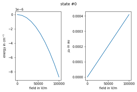
Owing to the dipole selection rules, if field is applied along the laboratory \(Z\) axis, it can only couple molecular states with the same \(m\) quantum number. We can exploit this in the above calculations by running a loop over \(m=-J_\text{max}..J_\text{max}\) where we extract a sub-matrix of the total tensor matrix representation corresponding to the current value of \(m\). To extract a sub-matrix corresponding to a basis spanned by a reduced subspace of quantum numbers, one
can use filter method (modifies tensor in place) or field.filter function (creates new object). The filter function accepts as arguments state quantum numbers \(J\), \(m\), and \(k\), symmetry, and energy and returns True or False depending on if the corresponding state needs to be included or excluded form the basis. Below is an example of how we can do it in the above Stark effect calculations
[13]:
from richmol.field import filter
import numpy as np
from richmol.convert_units import AUdip_x_Vm_to_invcm

def flt(**kw):
    """Filter function to select states with m = m_"""
    if 'm' in kw:
        m = kw['m']
        return m == m_
    return True

enr = {}
muz = {}
assign = {}

fz_grid = np.linspace(1, 1000*100, 10)  # field in units V/m

for m_ in range(-Jmax, Jmax+1):

    dip_m = filter(dip, bra=flt, ket=flt)
    h0_m = filter(h0, bra=flt, ket=flt)

    muz0 = dip_m.tomat(form="full", cart="z") # matrix representation of Z-dipole at zero field
    print(f"matrix dimensions for m = {m_}:", muz0.shape)

    enr[m_] = []
    muz[m_] = []
    assign[m_] = []

    for fz in fz_grid: # field in V/m

        field = [0, 0, fz] # X, Y, Z field components in V/m

        # Hamiltonian
        h = h0_m - dip_m * field * AUdip_x_Vm_to_invcm() # `AUdip_x_Vm_to_invcm` converts dipole(au) * field(V/m) into cm^-1

        # eigenproblem solution
        e, v = np.linalg.eigh(h.tomat(form='full', repres='dense'))

        # keep field-dressed energies
        enr[m_].append([elem for elem in e])

        # keep field-dressed matrix elements of Z-dipole
        muz[m_].append( np.dot(np.conjugate(v.T), muz0.dot(v)) )

        # keep state assignment by one leading basis fuction
        ind = np.argmax(np.abs(v), axis=0)
        assgn, _ = h0_m.assign(form="full")
        assign[m_].append( {key : [val[i] for i in ind] for key, val in assgn.items()} )
matrix dimensions for m = -5: (11, 11)
matrix dimensions for m = -4: (20, 20)
matrix dimensions for m = -3: (27, 27)
matrix dimensions for m = -2: (32, 32)
matrix dimensions for m = -1: (35, 35)
matrix dimensions for m = 0: (36, 36)
matrix dimensions for m = 1: (35, 35)
matrix dimensions for m = 2: (32, 32)
matrix dimensions for m = 3: (27, 27)
matrix dimensions for m = 4: (20, 20)
matrix dimensions for m = 5: (11, 11)
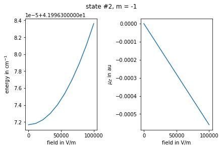
Plot the results for selected state index and \(m\)
[14]:
import matplotlib.pyplot as plt

# plot energies and dipoles vs field

enr = {m : np.array(val) for m, val in enr.items()}
muz = {m: np.array(val) for m, val in muz.items()}

istate = 2
m = -1

fig, (ax1, ax2) = plt.subplots(1,2, constrained_layout=True)
plt.suptitle(f"state #{istate}, m = {m}")
ax1.set_ylabel("energy in cm$^{-1}$")
ax1.set_xlabel("field in V/m")
ax2.set_ylabel("$\\mu_Z$ in au")
ax2.set_xlabel("field in V/m")
ax1.plot(fz_grid, enr[m][:, istate])
ax2.plot(fz_grid, muz[m][:, istate, istate].real)
plt.show()
Here is how we can print the assignment of a selected state for different values of field
[16]:
istate = 20
m = -3
for i, fz in enumerate(fz_grid):
    print("Fz =", fz, "J = ", assign[m][i]["J"][istate],
          "sym = ", assign[m][i]["sym"][istate],
          "m = ", assign[m][i]["m"][istate],
          "k = ", assign[m][i]["k"][istate])
Fz = 1.0 J =  4.0 sym =  A m =  -3 k =  ('4 0 0  0.612490', 487.7957659362319)
Fz = 11112.0 J =  4.0 sym =  A m =  -3 k =  ('4 0 0  0.612490', 487.7957659362319)
Fz = 22223.0 J =  4.0 sym =  A m =  -3 k =  ('4 0 0  0.612490', 487.7957659362319)
Fz = 33334.0 J =  4.0 sym =  A m =  -3 k =  ('4 0 0  0.612490', 487.7957659362319)
Fz = 44445.0 J =  4.0 sym =  A m =  -3 k =  ('4 0 0  0.612490', 487.7957659362319)
Fz = 55556.0 J =  4.0 sym =  A m =  -3 k =  ('4 0 0  0.612490', 487.7957659362319)
Fz = 66667.0 J =  4.0 sym =  A m =  -3 k =  ('4 0 0  0.612490', 487.7957659362319)
Fz = 77778.0 J =  4.0 sym =  A m =  -3 k =  ('4 0 0  0.612490', 487.7957659362319)
Fz = 88889.0 J =  4.0 sym =  A m =  -3 k =  ('4 0 0  0.612490', 487.7957659362319)
Fz = 100000.0 J =  4.0 sym =  A m =  -3 k =  ('4 0 0  0.612490', 487.7957659362319)
Time-dependent simulations
As an example, let’s simulate the laser induced ‘truncated-pulse’ alignment of linear OCS molecule.
[17]:
from richmol.rot import Molecule, solve, LabTensor
from richmol.tdse import TDSE
from richmol.convert_units import AUpol_x_Vm_to_invcm
from richmol.field import filter
import numpy as np
import matplotlib.pyplot as plt
To begin, compute the field-free energies, matrix elements of polarizability interaction tensor, and matrix elements of cosine and squared cosine functions of the Euler angle \(\theta\), that are used to quantify the degree of orientation and alignment, respectively
[18]:
ocs = Molecule()

ocs.XYZ = ("angstrom",
           "C",  0.0,  0.0,  -0.522939783141,
           "O",  0.0,  0.0,  -1.680839357,
           "S",  0.0,  0.0,  1.037160128)

# molecular-frame dipole moment (in au)
ocs.dip = [0, 0, -0.31093]

# molecular-frame polarizability tensor (in au)
ocs.pol = [[25.5778097, 0, 0], [0, 25.5778097, 0], [0, 0, 52.4651140]]

Jmax = 10
sol = solve(ocs, Jmax=Jmax)

# laboratory-frame dipole moment operator
dip = LabTensor(ocs.dip, sol)

# laboratory-frame polarizability tensor
pol = LabTensor(ocs.pol, sol)

# field-free Hamiltonian
h0 = LabTensor(ocs, sol)

# matrix elements of cos(theta)
cos = LabTensor("costheta", sol)

# matrix elements of cos^2(theta)
cos2 = LabTensor("cos2theta", sol) # NOTE: you need to add a constant factor 1/3 to get the true values
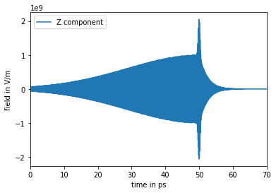
At the next step, we define the external electric field. Here we load it from file “trunc_pulse.txt”. The field in units V/cm has a single \(Z\) component and is defined on a time grid ranging from 0 to 300 picoseconds
[20]:
# truncated-pulse field
with open("trunc_pulse.txt", "r") as fl:
    field = np.array([[float(elem) for elem in line.split()[1:]] for line in fl]) # X, Y, Z field's components
    fl.seek(0)
    times = [float(line.split()[0]) for line in fl] # time grid

# convert field from V/cm to V/m
field *= 1e2

# plot Z component
plt.plot(times, field[:, 2], label="Z component")
plt.xlim([0,70]) # plot first 70 ps
plt.xlabel("time in ps")
plt.ylabel("field in V/m")
plt.legend()
plt.show()
Finally, we generate the initial states, set up the molecule-field interaction Hamiltonian and parameters of the time-dependent solution, and run the time propagation. For the initial states let’s assume a hypothetical temperature of \(T=0\) Kelvin and use eigenfunctions of the field-free operator h0 as the initial state vectors. Run dynamics from time zero to 200 ps with a time step of 10 fs
[21]:
tdse = TDSE(t_start=0, t_end=200, dt=0.01, t_units="ps", enr_units="invcm")

# initial states - Boltzmann-weighted eigenfunctions of `h0`, at T=0 K - only ground state
vecs = tdse.init_state(h0, temp=0)

# interaction Hamiltonian
H = -1/2 * pol * AUpol_x_Vm_to_invcm() # `AUpol_x_Vm_to_invcm` converts pol[au]*field[V/m] into [cm^-1]

# matrix elements of cos^2(theta)
cos2mat = cos2.tomat(form="full", cart="0")

cos2_expval = []

for i, t in enumerate(tdse.time_grid()):

    # apply field to Hamiltonian
    H.field([0, 0, field[i, 2]], thresh=1e2) # TODO: iprove performance of H * field operation

    # update vector
    vecs, t_ = tdse.update(H, H0=h0, vecs=vecs, matvec_lib='scipy')

    # expectation value of cos^2(theta)-1/3
    expval = sum(np.dot(np.conj(vecs[i][:]), cos2mat.dot(vecs[i][:])) for i in range(len(vecs)))
    cos2_expval.append(expval)

    if i % 1000 == 0:
        print(t, expval+1/3)
0.005 (0.33333335011354287-3.3881317890172014e-21j)
10.005 (0.34739158187693825-1.734723475976807e-18j)
20.005 (0.4213669350942997-1.0408340855860843e-17j)
30.005 (0.6609918655846478-2.7755575615628914e-17j)
40.005 (0.7625355344088344-2.7755575615628914e-17j)
50.005 (0.8276490955449676-2.7755575615628914e-17j)
60.005 (0.3821142205456442+5.551115123125783e-17j)
70.005 (0.19957705807366488-2.7755575615628914e-17j)
80.005 (0.6003828777604131+1.3877787807814457e-17j)
90.005 (0.2129905474603741+1.3877787807814457e-17j)
100.005 (0.5206370845603439-8.326672684688674e-17j)
110.005 (0.7736959532358003+2.7755575615628914e-17j)
120.005 (0.2798285070002713+2.7755575615628914e-17j)
130.005 (0.5766604584449334-1.3877787807814457e-17j)
140.005 (0.40216250912200846+5.551115123125783e-17j)
150.005 (0.12101474958572211-2.7755575615628914e-17j)
160.005 (0.6639581214246747-3.469446951953614e-17j)
170.005 (0.4410383542446014+3.8163916471489756e-17j)
180.005 (0.47123931234359556-6.938893903907228e-17j)
190.005 (0.7558934881925552+6.938893903907228e-17j)
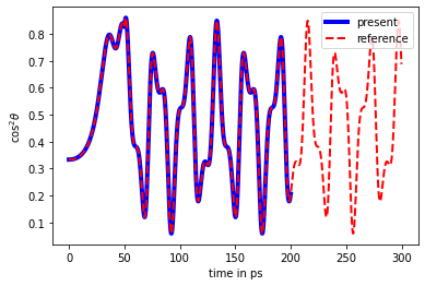
Plot the expectation value of \(\cos^2\theta\) and compare it with reference values (obtained with a different code)
[22]:
plt.plot([t for t in tdse.time_grid()], [elem.real + 1/3 for elem in cos2_expval], 'b', linewidth=4, label="present")

# compare with reference results
with open("trunc_pulse_cos2theta.txt", "r") as fl:
    cos2_expval_ref = np.array([float(line.split()[1]) for line in fl])
    fl.seek(0)
    times_ref = np.array([float(line.split()[0]) for line in fl])

plt.plot(times_ref, cos2_expval_ref, 'r--', linewidth=2, label="reference")
plt.xlabel("time in ps")
plt.ylabel("$\cos^2\\theta$")
plt.legend()
plt.show()
Since the alignment field is applied along the \(Z\) axis and thus couples only states with the same \(m\) quanta, we can split the full calculation into several once, each for different value of \(m=-J_\text{max}..J_\text{max}\). At the initial temperature of \(T=0\) K, simulations for \(m=0\) only are sufficient
[23]:
def flt(**kw):
    """Filter function to select states with m = m_"""
    if 'm' in kw:
        m = kw['m']
        return m == m_
    return True

cos2_expval = []

m_ = 0

h0_m = filter(h0, bra=flt, ket=flt)
pol_m = filter(pol, bra=flt, ket=flt)
cos2_m = filter(cos2, bra=flt, ket=flt)

tdse = TDSE(t_start=0, t_end=200, dt=0.01, t_units="ps", enr_units="invcm")

# initial states - Boltzmann-weighted eigenfunctions of `h0`, at T=0 K - only ground state
vecs = tdse.init_state(h0_m, temp=0)

# interaction Hamiltonian
H = -1/2 * pol_m * AUpol_x_Vm_to_invcm()

# matrix elements of cos^2(theta) in dense matrix representation
cos2mat = cos2_m.tomat(form="full", cart="0")

print(f"run m = {m_}, basis dimensions = {cos2mat.shape}")

for i, t in enumerate(tdse.time_grid()):

    # apply field to Hamiltonian
    H.field([0, 0, field[i, 2]], thresh=1e2) # TODO: iprove performance of H * field operation

    # update vector
    vecs, t_ = tdse.update(H, H0=h0_m, vecs=vecs, matvec_lib='scipy')

    # expectation value of cos^2(theta)-1/3
    expval = sum(np.dot(np.conj(vecs[i][:]), cos2mat.dot(vecs[i][:])) for i in range(len(vecs)))
    cos2_expval.append(expval)

    if i % 1000 == 0:
        print(m_, t, expval+1/3)
run m = 0, basis dimensions = (11, 11)
0 0.005 (0.33333335011354287-3.3881317890172014e-21j)
0 10.005 (0.34739158187693825+0j)
0 20.005 (0.4213669350942996-1.3877787807814457e-17j)
0 30.005 (0.6609918655846474+2.7755575615628914e-17j)
0 40.005 (0.7625355344088345-5.551115123125783e-17j)
0 50.005 (0.8276490955449656+2.7755575615628914e-17j)
0 60.005 (0.38211422054564265+5.551115123125783e-17j)
0 70.005 (0.19957705807366558-4.163336342344337e-17j)
0 80.005 (0.6003828777604128-1.3877787807814457e-17j)
0 90.005 (0.21299054746037452-6.938893903907228e-18j)
0 100.005 (0.5206370845603434-8.326672684688674e-17j)
0 110.005 (0.7736959532357975+5.551115123125783e-17j)
0 120.005 (0.2798285070002692+0j)
0 130.005 (0.576660458444932-1.3877787807814457e-17j)
0 140.005 (0.4021625091220066+2.7755575615628914e-17j)
0 150.005 (0.1210147495857242-4.163336342344337e-17j)
0 160.005 (0.6639581214246741-4.163336342344337e-17j)
0 170.005 (0.4410383542445989+5.204170427930421e-17j)
0 180.005 (0.4712393123435934-5.551115123125783e-17j)
0 190.005 (0.7558934881925505+2.7755575615628914e-17j)
Plot the expectation value of \(\cos^2\theta\) and compare with reference values
[24]:
plt.plot([t for t in tdse.time_grid()], [elem.real + 1/3 for elem in cos2_expval], 'b', linewidth=4, label="present")

# compare with reference results
with open("trunc_pulse_cos2theta.txt", "r") as fl:
    cos2_expval_ref = np.array([float(line.split()[1]) for line in fl])
    fl.seek(0)
    times_ref = np.array([float(line.split()[0]) for line in fl])

plt.plot(times_ref, cos2_expval_ref, 'r--', linewidth=2, label="reference")
plt.xlabel("time in ps")
plt.ylabel("$\cos^2\\theta$")
plt.legend()
plt.show()

[ ]: